Stanford researchers reported this May that robot policies scoring close to 90 percent in controlled simulation succeed at roughly 12 percent of real tasks; on a published peg-insertion benchmark one method managed 98.75 percent in simulation and 12.5 percent on hardware. The robots failing is not the interesting part. The interesting part is that nothing in the simulated score announced they would — the number was confident, precise, and silent about its own irrelevance. A method that cannot signal its own failure is worse than a mediocre one that can. Remember that; one of the ten methods below fails spectacularly, and the manner of its failure is the most reassuring thing in this post.
Psycho Killer
Today I am releasing psycho-killer, a toolkit for model-based diagnosis of dynamical systems. The name is a Talking Heads reference.
It is not a diagnosis algorithm and ships no opinion about which method you should use. It is a framework for diagnostic analytics: one system model, one shared set of fault scenarios, every applicable method run against them — filter-based and data-driven alike — scored on the same metrics. The output is not a diagnostic algorithm, it is a table you use to choose a diagnostic method, which is different and more useful.
It also ships a graphical IDE, and the GUI is the point. An engineer who has never opened a Python interpreter can load a model, inject a fault, watch the tanks respond, and get the comparison table out the other end — precisely the audience that ought to be doing model-based diagnosis and is currently being sold a chatbot instead.
The System
Three tanks in series, as in my May post on Lydia-NG. Water flows from tank 1 to 2 to 3 and out through three valves. Each valve has a commanded opening \(u_i\) and an actual condition \(f_i\), where 1.0 means it delivers what it was asked for. Three noisy pressure sensors are the only window in; nothing observes a valve directly.
Writing \(h_i\) for the level in tank \(i\), \(A_i\) for its cross-section, and
$$ \phi(\Delta h) \;=\; \frac{\Delta h}{\left(\Delta h^{2} + \varepsilon^{2}\right)^{1/4}} $$
for the regularised signed square root of a head difference — Torricelli, with \(\varepsilon\) smoothing the kink at zero so the integrator does not trip over it:
$$ \dot h_1 = \frac{1}{A_1}\Big(q_0 – f_1 u_1 k_1\,\phi(h_1-h_2)\Big) $$
$$ \dot h_2 = \frac{1}{A_2}\Big(f_1 u_1 k_1\,\phi(h_1-h_2) – f_2 u_2 k_2\,\phi(h_2-h_3)\Big) $$
$$ \dot h_3 = \frac{1}{A_3}\Big(f_2 u_2 k_2\,\phi(h_2-h_3) – f_3 u_3 k_3\,\phi(h_3)\Big) $$
with sensors reading \(p_i = h_i\,g\). Infer \(f_1, f_2, f_3\) from \(p_1, p_2, p_3\). It is a fair test because a closing valve does not merely dim the sensor nearest it — it backs pressure up behind and starves the tanks ahead, so the signature appears everywhere, differently shaped in each place.
Note \(\phi\). Its derivative runs from \(\varepsilon^{-1/2}\) near zero head difference down to roughly \(\frac{1}{2}|\Delta h|^{-1/2}\) when the tanks are far apart — orders of magnitude across the ordinary operating range. One of our ten methods is going to die on that.
The Run
Thirteen scenarios per split, 39 in total: one nominal, plus a ramp fault in each valve at each of four magnitudes. Ramps, not steps, because real valves do not fail instantaneously and a benchmark built on step changes flatters methods that detect step changes.
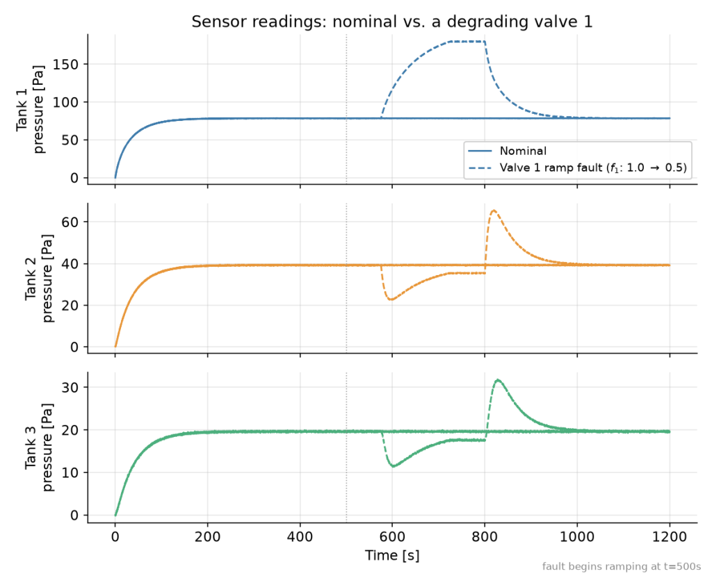
Valve 1 loses half its capacity for a few minutes, then recovers. That is all any method gets to see.
The filters consume raw readings online. The regressors cannot, so a rolling window over each sensor yields ten features apiece — min, max, mean and standard deviation in the time domain, plus six statistics over the window’s power spectrum.
I ran ten methods on one instance. Data-driven, trained once on the training scenarios: Decision Tree, Random Forest, Gradient Boosting, Linear and Ridge Regression, SVR, Multi-Layer Perceptron. Filter-based, with no training step at all, each carrying the ODEs forward in time and correcting against the sensors: Extended Kalman Filter, which linearises at each step; Unscented Kalman Filter, which propagates sample points through the exact nonlinear model instead; and a Particle Filter, deliberately under-provisioned at 50 particles (to save CPU time).
The Table
| Method | Family | Isolation accuracy | MSE | CPU/scenario |
|---|---|---|---|---|
| Random Forest | Data-driven | 0.975 | 0.003 | 0.037 s |
| Decision Tree | Data-driven | 0.968 | 0.0054 | 0.005 s |
| Ridge Regression | Data-driven | 0.844 | 0.0078 | 0.006 s |
| Linear Regression | Data-driven | 0.835 | 0.0074 | 0.006 s |
| Multi-Layer Perceptron | Data-driven | 0.762 | 0.0042 | 0.026 s |
| Gradient Boosting | Data-driven | 0.708 | 0.0031 | 0.006 s |
| SVR | Data-driven | 0.016 | 0.083 | 0.036 s |
| Unscented Kalman Filter | Filter-based | 0.486 | 0.0203 | 25.5 s |
| Extended Kalman Filter | Filter-based | 0.053 | 26.1 | 5.9 s |
| Particle Filter (50) | Filter-based | 0.017 | 155.4 | 134.4 s |
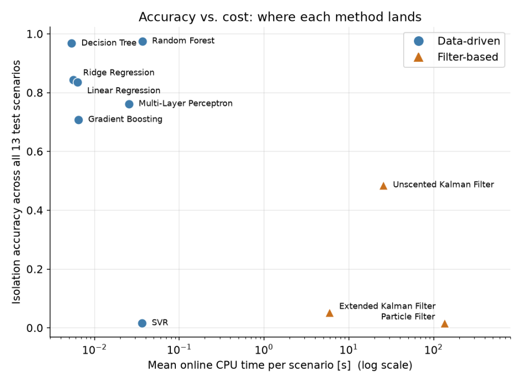
Two clusters, no overlap. The regressors pay for the model once, offline, in training; the filters pay every second of every scenario, because there is no training step to front-load the cost into. The whole study came to about half an hour of CPU on one machine — 81 percent of it the starved particle filter, while all seven data-driven methods together consumed under two seconds.
Three failures worth naming. The EKF diverges outright — that is \(\phi\) collecting its debt, the textbook failure of linearisation against strong nonlinearity, and exactly what the UKF exists to fix: same model, same scenarios, MSE some 1,300 times smaller. The particle filter was starved and behaved accordingly: 50 particles in a six-dimensional state space gives classic depletion, and it was still the most expensive thing on the board. SVR with sklearn defaults is no better than the starved filter. “Data-driven” is not a synonym for “accurate.”
Look closely at the Decision Tree, which wins the table. It holds flat at 1.0 through the entire descending ramp before jumping to the correct plateau, spikes to 0.2 when nothing is happening, and glitches once at \(t = 1090\,\text{s}\) in a fully recovered system. It is not tracking the dynamics. It is recognising a steady-state signature and binning it, extremely well. The UKF, at half the accuracy score, is estimating a continuous state and getting the shape roughly right. Different objects — which is why the toolkit reports eight metrics and not one.
Where the Labels Came From
The trees won, by a factor of two on accuracy and seven hundred on cost. This will surprise nobody who has worked in diagnosis. The interesting question is where the training data came from.
Those training scenarios do not exist in nature. Nobody has a record of a valve degrading to exactly 30 percent capacity with ground truth recorded alongside — as the maintenance vendors themselves concede, if pumps run ten years before failing you have almost no failure data. The regressors here were trained on scenarios simulated from the physical model, the same ODEs the filters integrate online. The model is load-bearing in both columns. The only thing that varies is when you pay for it.
Which makes the Random Forest a compiled, cached, lossy artefact of model-based diagnosis, fast for the reason a lookup table is fast. Strip the model away and there is no training set, and without a training set there is no forest. Yes, this is synthetic training data, and no, it is not the same activity as a frontier lab training on its own output: this generator is six equations, it conserves mass, its parameters were measured with a ruler and a stopwatch, and when it is wrong you can catch it against a physical system sitting right there. One of these arrangements can be audited by a second-year student with a bucket.
And the caveats have teeth. Every test fault came from the same generator as the training faults. Show that forest a stuck sensor, a leaking tank wall, or two simultaneous valve faults and it has nothing to generalize from, while the filters — never trained on anything — would at least attempt the right calculation. The forest cannot tell you why, cannot produce a certificate, and cannot report that it is out of its depth. It will simply answer.
Which returns us to those simulation scores. The EKF failed worse than almost anything here — and it failed legibly. The estimate climbed off the top of the chart and kept going. Nobody glancing at that plot on the way to lunch would mistake it for a diagnosis. It announced its own incompetence in the only language a diagnostic engine has, which is the shape of its output. A method that diverges is a method you can put an alarm on.
Next
psycho-killer is open source and the repository is live. Coming shortly: a video of the GUI doing all of the above, and guidelines for building it and pointing it at a system of your own.
After that, the direction of travel. Component-based hierarchical models, in the manner of Modelica — a plant assembled from reusable, nested components rather than hand-written as one flat set of equations, which is the only way this scales past three tanks to a refinery. A distributed web version, which will be paid, because the compute is not free and neither am I. And code generation: once the table tells you which method wins on your system, you get a deployable implementation of it rather than a recommendation. That is the whole arc — measure honestly, choose on evidence, ship the winner.
Ten methods. One model. Eight metrics. Half an hour of CPU, no gigawatts, and a table somebody else can check.
Ceterum censeo slopem esse delendam.
(Cato the Elder ended every speech in the Roman Senate with “Carthage must be destroyed” — regardless of the topic. This is that, but for AI slop.)
Repository: psycho-killer
What those two studies share is not “AI is bad.” It is that a diagnostic method which cannot signal its own failure is worse than a mediocre one that can. Remember that; one of the ten methods below fails spectacularly, and the manner of its failure is the most reassuring thing in this post.
Leave a Reply